ECE 4160 Fast Robots
Raphael Fortuna
Lab reports made by Raphael Fortuna @ rafCodes Hosted on GitHub Pages — Theme by mattgraham
Home
Lab 10: Grid Localization using Bayes Filter
Summary
In this lab, I implemented grid localization using a Bayes Filter in the provided simulation. This uses probabilistic methods for localization as non-probabilistic can be unreliable and probabilistic methods seek to improve the accuracy of the robotics location.
Prelab
The prelab involved going through the provided background information and reviewing the Bayes Filter algorithm. The background information included the terminology for robot localization, grid localization, gaussian model for sensor measurement noise, and motion model for relative movement changes between time steps.
The grid localization is partitioned into a discretized x, y, and theta space – 12, 8, and 18 respectively – to allow for a short computation time and each x, y, theta triple corresponds to a robot location and orientation in the space and the probability of it being there, with the sum over all triples being 1.
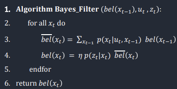
The Bayes filter algorithm is a cycle of prediction of where the robot thinks it is based on its movement (prior belief) followed by an update step to reduce the uncertainty of where the robot thinks it is. The update step uses the data collected by the sensors to do this.
The image below shows the equation for the Bayes filter algorithm from lecture 21.

Codebase
The code being used was from the provided simulation in class with two additions – importing numpy and math for the Bayes filter calculations. The file used for the lab was provided and had five classes: a commander class to interface with the simulator and plotting, a VirtualRobot class to interface with the robot and its sensors, a mapper class that bundles information and functions for the grid map, BaseLocalization bundling localization functions and ToF data collection, and the Trajectory class that has a path that it manages and has the robot execute. I did not have to modify the Trajectory as my robot did not crash while executing the trajectory.
Localization Task: Compute Control
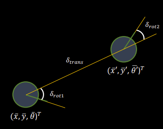
The first function was compute_control that took in the current and previous pose of the robot and got the control information using the odometry motion model. Each pose is composed of a x, y, and yaw the final output should be a rotation, translation, and rotation that described the change in position and direction between the two poses. The image below from lecture 17 describes how the rotations and translations interact with the two poses.
The first rotation is to move from the initial direction to the direction of the other pose.
The translation is the movement between the first and second pose.
And the second rotation is to align the robot to the correct direction at the second pose. I found the difference between the current angle and the angle – as well as distance - needed to translate from pose 1 to pose 2 and then got the last rotation from what the final orientation should be.

Localization Task: Odometry Motion Model
The odom_motion_model function was used in finding the prior beliefs of the Bayes Filter based on the movement of the robot from one pose to another through prediction. We used the necessary control action, u, and the actual_u computed from the two poses to determine how likely the transition was from the previous pose to the current pose though multiple gaussian functions multiplied together and described below from the lab guide:

Translating this into code is shown below:
Localization Task: Updating Prior Belief
This function was used to update all the prior beliefs, bel bar, given a previous location and looked the probability of traveling to every location from the given previous location. It used the odom_motion_model function for getting the transition probability. The photo below shows what section of the Bayes Filter is being computed from lecture 21.

The code for this is shown below:
Localization Task: Prediction Step
The next function iterated over all the poses with their previous beliefs and updated the prior belief using the previous function. This is the prediction step of the Bayes Filter. When iterating though the different locations, the beliefs that are under .0001 are skipped since those are too small to have an impact and will be near 0 when updating the prior belief with them. At the end, the previous beliefs are normalized since it is a probability distribution and must sum to 0.
Localization Task: Sensor Model
Moving on to the update step of the Bayes Filter, this next function is used to get the likelihood of getting each of the sensor’s measurements given what the actual measurements would be for a given certain location’s pre-cached sensor data. This is to determine what locations would the sensor measurements be the most likely to come from, p(z|t).
Localization Task: Update Step
The update step is the second half of the Bayes Filter and updates the previous beliefs, with the equation it describes shown below from lecture 21.

Each point was iterated over and updated using the sensor model to first get the probability p(z|x) and then multiplied with the prediction step belief probability for that location to get the new belief for that location. After all points had been updated, the belief was normalized so that the total probability of the belief was 1.
Running the Bayes Filter Task
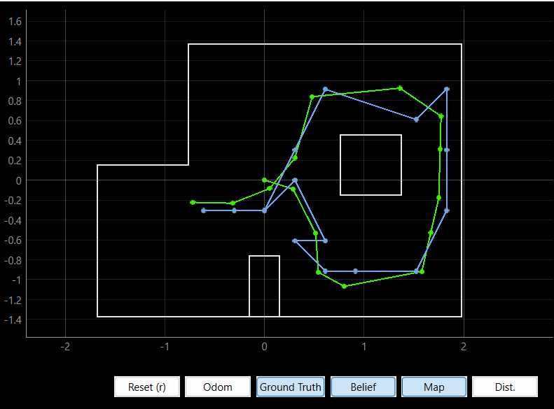
I ran the Bayes Filter over the pre-programmed trajectory and recorded the plotter, simulation, and Jupyter notebook output. In the plotter, the green line was the ground truth of the robot, blue was the predicted location from the bayes filter, and the odometry readings were in red. The second video had squares on the map that represented that probability the robot was in that location, with white having the highest probability of having the robot. Below I have a photo of the completed trajectory and the two videos of the robot driving around.
